GalaxyGAN

Created by: Armand Mousavi, Karman Singh, and Matthew Foss

UW student project for CSE490G1

Try the demo out for yourself

Video

Abstract/Background

A Generative Adversarial Network can be broken down into three parts: learn a generative model, train a model in an adversarial setting, and use deep neural networks. In a GAN there is the generator and the discriminator. The Generator creates fake images to input into the discriminator. The discriminator takes two images, one real and one fake. The discriminator’s job is to decide whether the image is fake or real. The generative model tries to maximize the probability of fooling the discriminator while the discriminator tries to maximize the probability of the sample being from the real dataset. Pictured below is a basic representation of a GAN, credit from

source

The GalaxyGAN implementation follows this methodology. GalaxyGAN was designed to create fake images to fool the discriminator.

Problem statement

We want to see if we can use a Generative Adversarial Network to produce new images of fake galaxies using a comprehensive dataset of colored galaxy images and do it in a way that we didn’t have to train the model for more than a couple days.

Related work

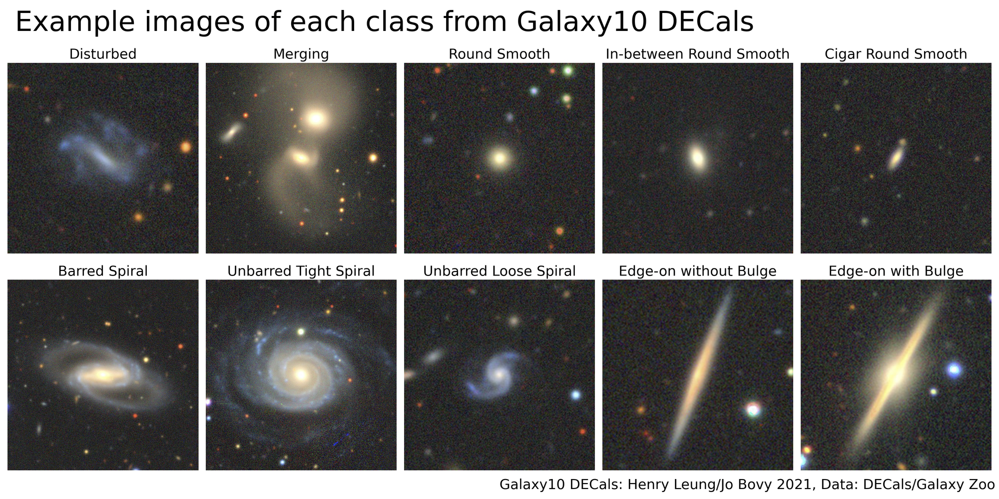
We talked about using GAN and the best ways to utilize this network. We searched many different websites with datasets. The dataset we used was a relatively large set of galaxy images called Galaxy10 DECals from this website. The Galaxy10 DECals is an improved version of Galaxy10. The Galaxy10 dataset was created with the Galaxy Zoo data release where volunteers classified around 270K of Sloan Digital Sky Survey, SDSS, galaxy images. GZ later utilized DESI Legacy Imaging Surveys to create the new and improved version Galaxy10 DECals.

Galaxy10 dataset (17736 images)

• Class 0 (1081 images): Disturbed Galaxies
• Class 1 (1853 images): Merging Galaxies
• Class 2 (2645 images): Round Smooth Galaxies
• Class 3 (2027 images): In-between Round Smooth Galaxies
• Class 4 ( 334 images): Cigar Shaped Smooth Galaxies
• Class 5 (2043 images): Barred Spiral Galaxies
• Class 6 (1829 images): Unbarred Tight Spiral Galaxies
• Class 7 (2628 images): Unbarred Loose Spiral Galaxies
• Class 8 (1423 images): Edge-on Galaxies without Bulge
• Class 9 (1873 images): Edge-on Galaxies with Bulge

Methodology

We referred to the tutorials for guidance from here and from here.

Before working with the data for the final model we downsized all of the images from the original dataset. The 256x256 images required a larger model that took an extreme amount of time to train on and more RAM than we had available on colab to comfortably work with.

We first define the discriminator model, which needs to take a sample image from our dataset as input and output a classification prediction as to whether the sample is real or fake. The inputs are three color channels and 128 by 128 pixels in size. The model has a normal convolutional layer followed by five convolutional layers using a stride of 2 by 2 to downsample the input image. The model has no pooling layers and a single node in the output layer with the sigmoid activation function to predict whether the input sample is real or fake. The model is trained to minimize the binary cross entropy loss function, which is suitable for binary classification. We use the industry best practice with the LeakyReLU instead of ReLU, and the Adam version of stochastic gradient descent with a learning rate of 0.0002 and a momentum of 0.5

The generator model is responsible for creating new, but fake images and does this by taking a point from the latent space as input and outputting a square color image. We don’t want just one low-resolution version of the image, but many parallel interpretations of the input. So, the first hidden layer, the Dense layer, needs enough nodes for multiple versions of the output image, such as 256. The activations from these nodes can be reshaped into an image shape to pass into the convolutional layer, such as 256 different 4 by 4 feature maps. Now we need to upsample the low-resolution image to a higher resolution version of the image. We will use Conv2DTranspose to reverse pool and convolute. We configure the Conv2DTranspose layer with stride of 2 by 2 and quadruple the area of the input feature maps by doubling the width and height. We up sample five times to reach the required output image size of 128 by 128. We use the LeakyReLU activation function again as best practice for training GAN models. The output layer of the model is a Conv2D with three filters for the required three channels and kernel size of 3 by 3. Finally a tanh activation is used to ensure the output values are in the range [-1, 1].

For generating real samples, we will just take the training dataset and select a random subsample of images. We need to generate new points in the latent space and the array of random numbers then reshape into samples, which are then used as input to the generator model. We need to generate images composed of random pixel values for the generate fake samples function, which takes in the generator model as an argument.

Here you can see the full model for the discriminator:

As well as the model for the generator:

Experiments/evaluation

You can check out our final notebook we used to train our model here

When evaluating the Generative Adversarial Network, there isn’t really an objective error score for the generated images. The images will need to subjectively be evaluated. Also the adversarial nature of the training means the generator is changing after each batch and the subjective quality of the images may improve or degrade with further updates. To handle this, first we periodically evaluate the classification accuracy of the discriminator on real and fake images, second we periodically generate many images and save them for review, and third we periodically save the generator model. If we train the GAN over many epochs, we would be able to get many snapshots of the model and choose the best models, once reviewed for performance.

We define a function for summarizing the performance of the discriminator model. This function takes a sample of real galaxy images and generates the same number of fake galaxy images with the generator model and then evaluates the classification accuracy of the discriminator model and reports the score for each sample.

This is an example of the loss values on real images and fake generated images for the discriminator and the generator for epoch 26

1
2
3
4
5
6
7
8
9
10

>26, 1/138, d1=0.29638204, d2=0.32488263 g=3.45844007
>26, 2/138, d1=0.45061448, d2=0.88800186 g=4.71526003
>26, 3/138, d1=1.16259015, d2=0.06006718 g=4.13229275
>26, 4/138, d1=0.72051704, d2=0.09301022 g=2.78597784
>26, 5/138, d1=0.81719440, d2=0.22286285 g=2.34299660 … … …
>26, 134/138, d1=1.59510779, d2=0.09820783 g=2.37885666
>26, 135/138, d1=0.35758907, d2=0.54601729 g=2.40457916
>26, 136/138, d1=0.22124308, d2=0.10850765 g=2.61518002
>26, 137/138, d1=0.18373565, d2=0.13180479 g=2.34858227
>26, 138/138, d1=0.02594333, d2=0.20959115 g=2.79657221

This is an example of the model’s accuracy score for epoch 26 based on the discriminators ability to differentiate

1

>Accuracy real: 94%, fake: 100%

This is an example of the image produced by the model for epoch 26

Results

Epoch 11

Epoch 12

Epoch 13

Epoch 14

Epoch 15

The results after the first training process for 15 epochs yielded the following results and we can see that the quality of the images are not consecutively increasing and from my understanding, Epoch 13 out of the last five epochs had the best result with the least amount of noise in comparison to the colorful galaxy center. At this stage the galaxy isn’t very detailed and more like a cloud of color, with a ton of noise and repetition of small sections, introducing patterns.

Epoch 41

Epoch 42

Epoch 43

Epoch 44

And finally… Epoch 45

These are the results after the second training process for an additional 35 epochs. We can see that the quality does get better and there is more detail but we can see issues with repeated patterns in Epoch 41 and 42. The last three are fairly good representations of galaxies, where Epoch 43 has a very clean image, with a detailed galaxy center with little outside noise. Epoch 44 has a bit of a problem with the patterns of the outside of the galaxy with the red spots but the galaxy center is really rich in color and detail. Epoch 45 is the combination of the last two, where the center is colorful and clear and the surrounding is pretty clean with minimal noise.

Final Thoughts

With more time we would definitely continue training this network, maybe on some persistent computer for at least a week. This would also allow us to attempt to generate original sized images at 256x256. It would also be wise for us to try new models like to add batch normalization layers to the layers of the discriminator which is quite easy with keras.

Thank you again to the whole team and to you for reading our report.